Classifying Paintings through Deep Learning

Using ResNets to revive an old class project

Featured photo by Clem Onojeghuo on Pexels.com

Back in college, I did a class project where I used computer vision techniques for the first time. I wanted to classify paintings to genres — abstract, realist, impressionist, baroque. It was the age before deep learning, and so the features available were histograms, blobs, and edges. I haven’t heard yet of SIFT and bag-of-words for images then, so the project was very basic. But you had to start somewhere, and that was already very exciting for me. Matlab then was the pinnacle of machine learning. Today, we know all about the numpy stack and deep learning frameworks. Wouldn’t it be fun to revisit an old project?

You can check out the notebooks from Github here. You can also check the Kaggle Notebooks here.

The Challenge

We’re using the Historic Art dataset from Kaggle. It’s a large collection of artworks and their metadata. Other than paintings, there are sculptures, architecture, graphic design, and even ancient pottery and tapestry. In the paintings department, we have the works of different artists, from Donatello to Van Gogh. It spans several periods, from Medieval to Impressionism. The paintings number 33,611 from 5565 painters. In this exercise, I filter only a few painters I’m familiar with. Note that this selection is completely arbitrary:

Period	Artist	# of Samples
Medieval	Giotto	550
	Duccio	170
Early Renaissance	Fra Angelico	244
	Botticelli	204
Northern Renaissance	Bruegel, the Elder	223
	Bosch	162
Baroque	Rembrandt	539
	Caravaggio	185
Romanticism	Goya	197
	Delacroix	105
Impressionism	Van Gogh	420
	Monet	198

Note that some of the samples are actually details of a larger work. For example, the Garden of Earthly Delights by Bosch has several zoomed-in samples in the data, depicting scenes within the piece.

I want to make a classifier that distinguishes the different periods. To do so, I will use PyTorch Lightning to create our model and training routines. I will compare ResNet18, 34, and 50 if there is a difference in accuracy. As an added challenge, I also want to try out multi-task learning, with predicting the period and the artists simultaneously to hopefully steer the training in a positive direction. Finally, I want to visualize what the network is doing beyond the metrics. I want to see gradient maps to uncover what latent features the network processes.

Lastly, a disclaimer. I’m not an expert in art history or any academic history. I’m simply a museum-goer with a taste for these beautiful paintings. So I’m afraid I can’t explain all the nuances of the Renaissance, and the fun elements of the impressionist movement.

Code On

First, we start with the DataLoader. I’m also defining a SquarePad transformer, based here, to keep the ratio of the image dimensions.

	class SquarePad:
	def __call__(self, image):
	w, h = image.size
	max_wh = np.max([w, h])
	hp = int((max_wh – w) / 2)
	vp = int((max_wh – h) / 2)
	padding = (hp, vp, hp, vp)
	return torchvision.transforms.functional.pad(image, padding, 0, 'constant')
	class ArtPeriodDataSet(Dataset):
	def __init__(self, dataframe, img_dir, transform=None, target_transform=None):
	self.dataframe = dataframe.copy()
	self.img_dir = img_dir
	# eliminate non-existing files
	print("Eliminate non-existing files")
	for idx, row in tqdm(dataframe.iterrows(), total=len(dataframe)):
	path = f'{img_dir}/{row["ID"]}.jpg'
	if not os.path.exists(path):
	self.dataframe.drop(idx, inplace=True)
	print("Dropping", path)
	# encode brands
	self.label_encoder = LabelEncoder()
	labels_encoded = self.label_encoder.fit_transform(self.dataframe["period"])
	self.dataframe["period_encoded"] = labels_encoded
	self.classes = self.label_encoder.classes_
	self.img_dir = img_dir
	self.transform = transform
	self.target_transform = target_transform
	def __len__(self):
	return len(self.dataframe)
	def __getitem__(self, idx):
	img_path = f'{self.img_dir}/{self.dataframe.iloc[idx]["ID"]}.jpg'
	image = PIL.Image.open(img_path).convert('RGB')
	label = self.dataframe.iloc[idx]["period_encoded"]
	if self.transform:
	image = self.transform(image)
	if self.target_transform:
	label = self.target_transform(label)
	return image, label

view raw pytorch_paintings_dataset.py hosted with ❤ by GitHub

My transformations and augmentations are standard. We use square padding, resize to 256, center crop to 224, then normalize via ImageNet mean and standard deviation. For the train, validation, and test splits, I have the following summary:

Label	Train	Val	Test	Total
Baroque	664	30	30	724
Medieval	661	30	30	721
Impressionism	558	30	30	618
Early Renaissance	388	30	30	448
Northern Renaissance	325	30	30	385
Romanticism	242	30	30	302

We are using pre-trained ResNet models from torchvision. The definition and training routines use PyTorch Lightning, which personally, makes the code more beautiful and more organized.

	class LightningResNet(pl.LightningModule):
	def __init__(self, net_pretrained, device='cpu', criterion = F.cross_entropy,
	num_classes = 4, optimizer = None, scheduler = None):
	super().__init__()
	self.net = net_pretrained
	# set top to number of classes
	num_ftrs = self.net.fc.in_features
	self.net.fc = nn.Linear(num_ftrs, num_classes)
	self.criterion = criterion
	self.optimizer = optimizer
	self.scheduler = scheduler
	def forward(self, x):
	return self.net(x)
	@torch.no_grad()
	def accuracy(self, outputs, labels):
	_, preds = torch.max(outputs, dim=1)
	return torch.tensor(torch.sum(preds == labels).item() / len(preds))
	def training_step(self, batch, batch_idx):
	loss, acc = self._shared_eval_step(batch, batch_idx)
	metrics = {'train_loss': loss, 'train_accuracy': acc}
	self.log_dict(metrics)
	return {'loss': loss, "train_accuracy" : acc}
	def test_step(self, batch, batch_idx):
	with torch.no_grad():
	loss, acc = self._shared_eval_step(batch, batch_idx)
	metrics = {"test_acc": acc, "test_loss": loss}
	self.log_dict(metrics)
	return metrics
	def validation_step(self, batch, batch_idx):
	with torch.no_grad():
	loss, acc = self._shared_eval_step(batch, batch_idx)
	metrics = {'val_loss': loss, 'val_accuracy': acc}
	self.log_dict(metrics, prog_bar=True)
	return metrics
	def _shared_eval_step(self, batch, batch_idx):
	images, labels = batch
	out = self(images)
	loss = self.criterion(out, labels)
	accu = self.accuracy(out,labels)
	return loss, accu
	def configure_optimizers(self):
	if not self.optimizer:
	optimizer = optim.SGD(self.net.parameters(), lr=0.001, momentum=0.9)
	plateau_scheduler = optim.lr_scheduler.ReduceLROnPlateau(optimizer, mode='max', patience=3, verbose=True)
	return {
	"optimizer": optimizer,
	"lr_scheduler": {
	"scheduler": plateau_scheduler,
	"monitor": "val_accuracy"
	}
	}
	else:
	return {
	"optimizer" : self.optimizer,
	"lr_scheduler": {
	"scheduler": self.scheduler,
	"monitor": "val_loss"
	}
	}
	# load data loaders and parameters
	# …
	# get pretrained
	net = models.resnet18(pretrained=True)
	# create and load the optimizers
	optimizer = optim.SGD(net.parameters(), lr=lr, momentum=momentum)
	plateau_scheduler = optim.lr_scheduler.ReduceLROnPlateau(optimizer, mode='min', patience=plateau_lr_decrease, verbose=True)
	clf_resnet18 = LightningResNet(net, num_classes=len(classes), device=device, optimizer = optimizer, scheduler=plateau_scheduler)
	# prepare callbacks
	callbacks = [pl.callbacks.EarlyStopping("val_accuracy", mode='max', patience=patience)]
	logger = pl.loggers.CSVLogger("logs", name="resnet18-a1-transfer-logs", version=0)
	# prepare trainer and launch!
	trainer_resnet18 = pl.Trainer(accelerator="auto", gpus=1, callbacks=callbacks, max_epochs=max_epochs, log_every_n_steps=1, logger=logger)
	trainer_resnet18.fit(model=clf_resnet18, train_dataloaders=dataloaders['train'], val_dataloaders = dataloaders['val'])

view raw pytorch_paintings_model.py hosted with ❤ by GitHub

In one set of runs, I freeze the feature extraction layers and only train the heads of the models. This is to ensure the model does not ‘catastrophically forget’ the breadth of its earlier ImageNet training. I repeat the runs for ResNet34 and 50 to find out the best classifier. To squeeze out a little extra performance, I then enable the training of all layers, while keeping the learning rate very low.

In another set of runs, I try out multi-task classification. The first task is predicting the period and the second is the artist. To do this, you must modify the DataLoader to output two labels while also modifying the forward function of your PyTorch Lightning model. Here’s the relevant snippet:

	# following https://towardsdatascience.com/multilabel-classification-with-pytorch-in-5-minutes-a4fa8993cbc7
	class LightningResNetMultiLabel(pl.LightningModule):
	def __init__(self, net, n_period, n_artists, criterion = F.cross_entropy, optimizer = None, scheduler = None, dropout_p = 0., lr=0.001, freeze_net=False):
	super().__init__()
	self.net = net
	self.feature_extractor = nn.Sequential(*(list(self.net.children())[:–1]))
	if freeze_net:
	for param in self.net.parameters():
	param.requires_grad = False
	num_ftrs = net.fc.in_features
	self.period_fc = nn.Sequential(
	nn.Dropout(p=dropout_p),
	nn.Linear(in_features=num_ftrs, out_features=n_period)
	)
	self.artist_fc = nn.Sequential(
	nn.Dropout(p=dropout_p),
	nn.Linear(in_features=num_ftrs, out_features=n_artists)
	)
	self.loss_func = criterion
	self.optimizer = optimizer
	self.scheduler = scheduler
	self.learning_rate = lr
	def criterion(self, loss_func, outputs, inputs):
	losses = 0
	for i, key in enumerate(outputs):
	losses += loss_func(outputs[key], inputs[f'{key}_label'])
	return losses
	def forward(self, x):
	x = self.feature_extractor(x)
	x = torch.flatten(x, 1)
	return {
	'period': self.period_fc(x),
	'artist': self.artist_fc(x),
	}
	def _shared_eval_step(self, batch, batch_idx):
	images = batch["image"]
	period_labels = batch["period_label"]
	artist_labels = batch["artist_label"]
	out = self(images)
	out_period = out["period"]
	out_artist = out["artist"]
	loss = self.criterion(self.loss_func, out, batch)
	period_accu = self.accuracy(out_period, period_labels)
	artist_accu = self.accuracy(out_artist, artist_labels)

view raw pytorch_multitask_paintings.py hosted with ❤ by GitHub

It’s also helpful to know that PyTorch Lightning comes with its own learning rate finder. Simply use the auto_lr_find=True in the Trainer and use trainer_resnet18.tune. I used this in the multi-task experiments and the runs that did not involve freezing the feature extractor layers.

Evaluation

Run	Model	Loss	Accuracy
1	ResNet 18 (11.4 M params)	0.697	0.722
2	ResNet 34 (21.5 M params)	0.720	0.722
3	ResNet 50 (23.9 params)	0.730	0.733
4	ResNet 18 – Train All Layers after top training	0.499	0.789
5	ResNet 18 – Train All Layers immediately	1.018	0.600
6	ResNet 18 – Multi-Task	4.947	0.556
7	ResNet 34- Multi-Task	4.867	0.472

For Runs 1-3, the metrics are nearly the same, so it proves we can use the simplest model (11.4 M parameters counts as simplest in this case!). I reach the best metrics in Run 4. Run 5, the method that involved training all the layers off-the-shelf, proves a little less accurate than the best run. Runs 6-7 are a letdown, as their accuracy on the artists is also dismal.

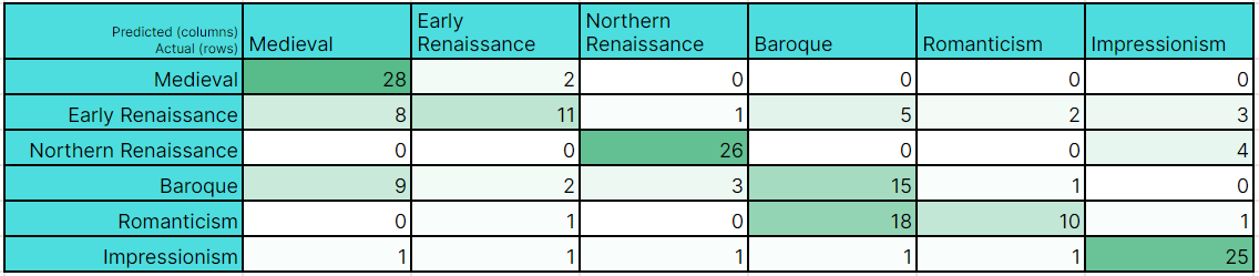
The confusion matrix reveals some difficult examples of cross-over from adjacent periods. For example, early renaissance works are predicted as medieval, and romanticism is predicted most of the time as baroque. I’m not sure why some baroque pieces are predicted as medieval, however. Perhaps a gallery of errors will help.

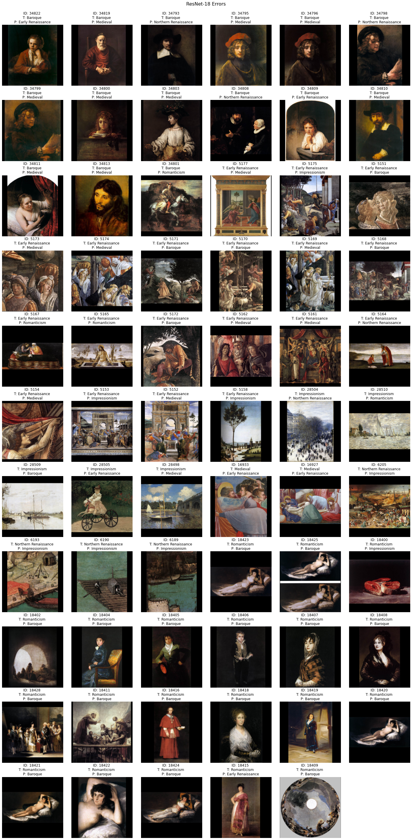
Got it. The errors of the romanticism period are portraits, which are very popular in the baroque period. As for the errors of the baroque period being misclassified as medieval, I’m not sure. Perhaps it sees something religious in nature in the long hairs. It should be noted though that these are mostly portraits of Titus, Rembrandt’s only son that reached adulthood.

Visualizations

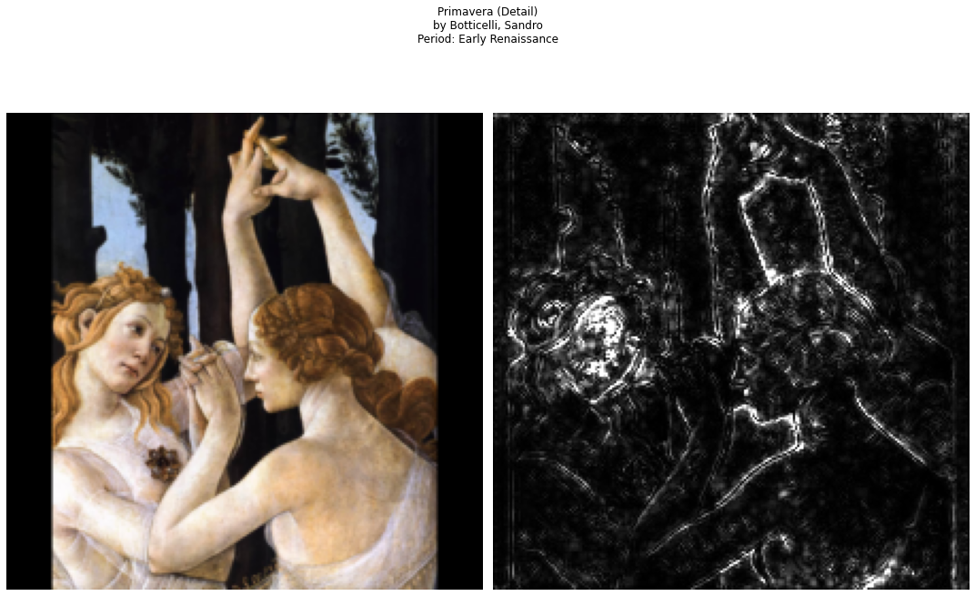
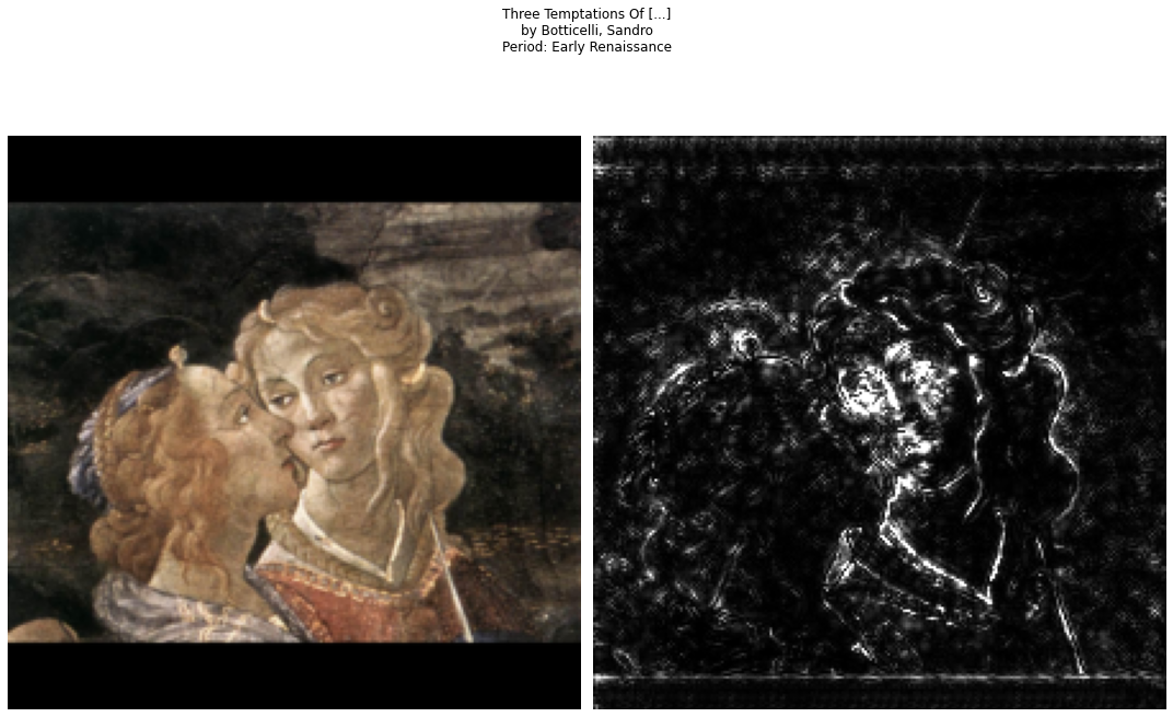
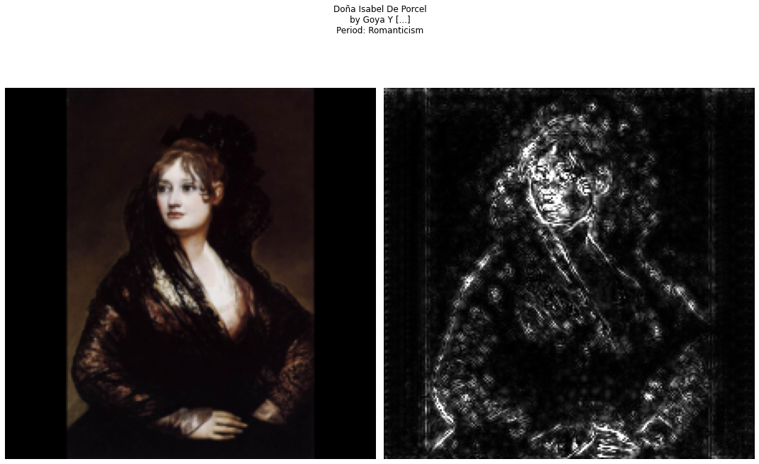
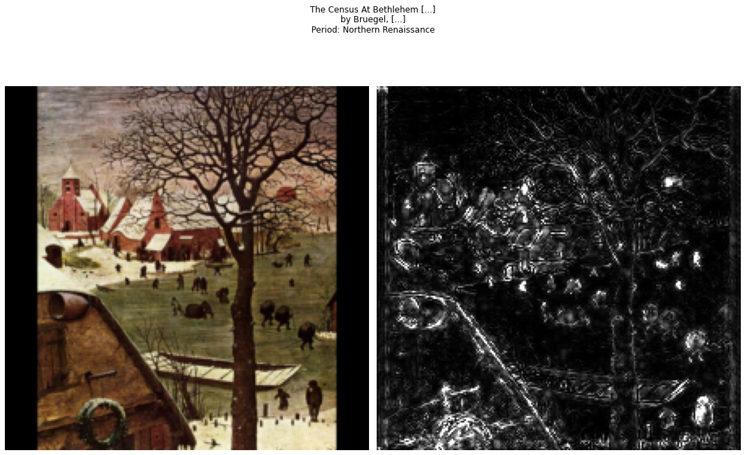
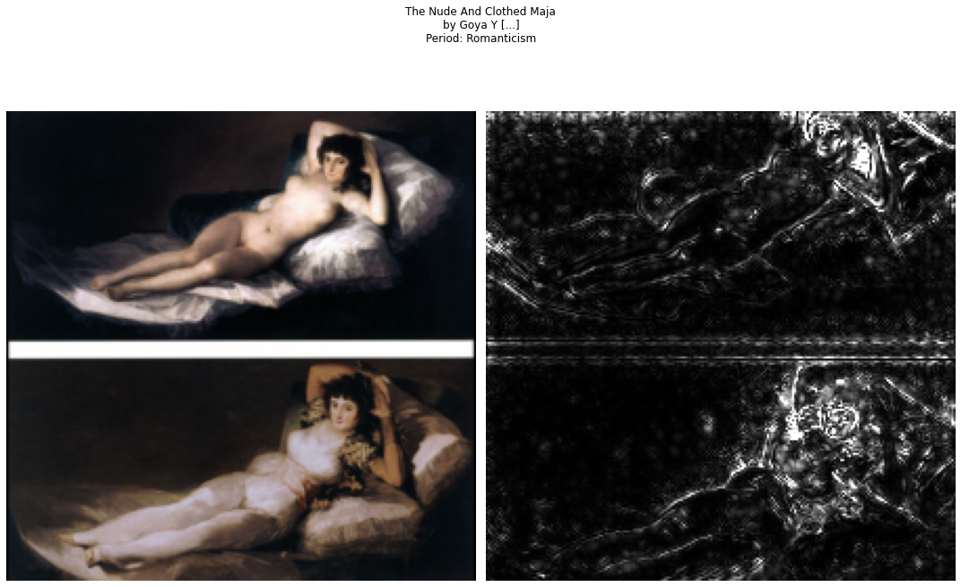
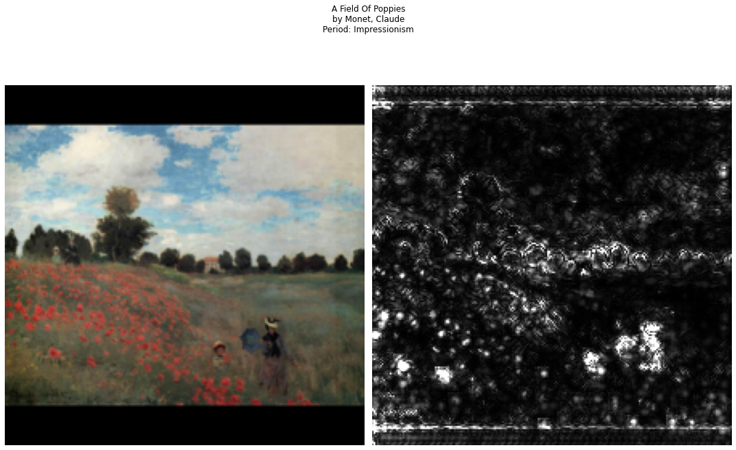
Here, I use the best run’s parameters to visualize what the network is doing. After some fiddling around, I landed on using Guided Backpropagation. I have the following for consideration:

Update: Train on All Paintings

I did a follow-up set of experiments to see how well ResNet-18 will work with the whole 33,000 paintings data. I did stratified sampling. 20% of the total samples go to validation and another 20% for the test set.

Period	train	val	test	total
Baroque	7240	1810	2263	11313
Early Renaissance	2537	634	793	3964
Northern Renaissance	2068	517	646	3231
Mannerism	1936	484	605	3025
Impressionism	1458	365	456	2279
Medieval	1418	355	443	2216
High Renaissance	1358	340	425	2123
Rococo	1301	325	407	2033
Romanticism	1041	260	325	1626
Realism	609	152	190	951
Neoclassicism	389	97	121	607
Art Nouveau	155	39	49	243

For these runs, I freeze only a part of ResNet, and let it train on the rest. Below, run 1 means the first block is frozen and the rest are trained. Run 2 means that the first and second block is frozen. And so on. This form of transfer learning keeps the bottom features active from the larger ImageNet data, while creating new hierarchies of features higher up the model. Here’s the Kaggle Notebook.

Run	Model	Loss	Accuracy
1	ResNet 18 – Freeze up to 1st	2.092	0.380
2	ResNet 18 – Freeze up to 2nd	1.777	0.524
3	ResNet 18 – 3rd	1.966	0.552
4	ResNet 18 – 4th	2.612	0.069

There are significant differences, and in this case, it looks like freezing up to the 2nd or 3rd block will both work well. This means that the higher convolutional blocks are free to create features that are well suited for this domain.

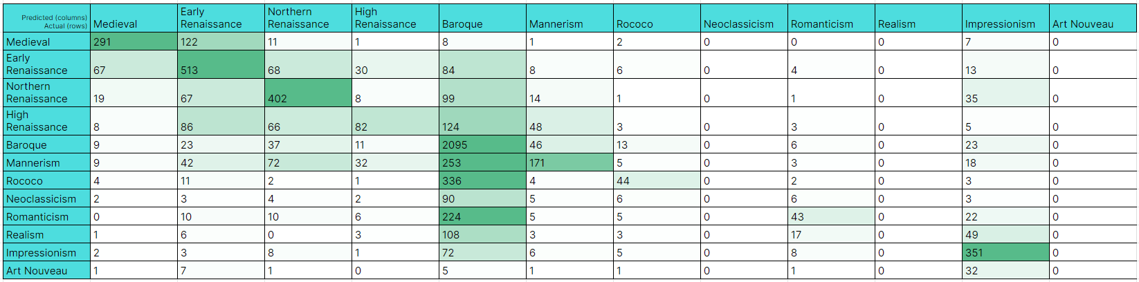
Like the confusion matrix of our first experiments, the misclassification tends to be on adjacent periods. In this case, there are classes with zero correct predictions. Neoclassicism, realism, and art nouveau are not recognized at all while baroque is predicted everywhere. Perhaps this is expected since the class distribution tends heavily on it.

Learnings

This has been a fun exercise. I’m quite proud of where I stand today, in a field that has become very active since the last time I used traditional computer vision features. I wish I can pat my younger self on the back and say to plow on — the field gets very exciting!

Some learnings, to close:

• The simplest model wins, but perhaps if I use the larger paintings data, then the capacity of ResNet50 wins.
• For this exercise, I find that PyTorch Lightning is a big boost to your training. It makes your model and computation organized into tidy and reusable blocks.
• Dropping the learned weights (or at least part of it), then retraining on all the images from all artists might also work well.
• I did not get the multi-task learning to work well. Perhaps more data is required for this. Or more tuning.
• For visualization, I’ve tried image generation, but the images did not make sense. For that to fly, GANs are the way to go for sure.

Thanks for reading!