
The State Farm Distracted Driver Detection competition just this week. It involves using machine learning for recognizing different forms of distracted drivers, such as talking on a mobile phone, texting and drinking. It is especially relevant for today’s sad situation of hundreds of thousands of injuries involving car accidents.
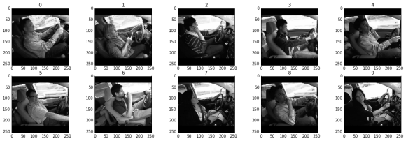
This competition features a large dataset of 640×480 images separated into standardized training and test sets. Immediately, the obvious solution was to use convolutional neural networks, which captures spatial characteristics of images, and transform them into hierarchical invariant features for classification. But many questions remain. What kind of architecture? How do we define the optimization algorithm?
First Solutions
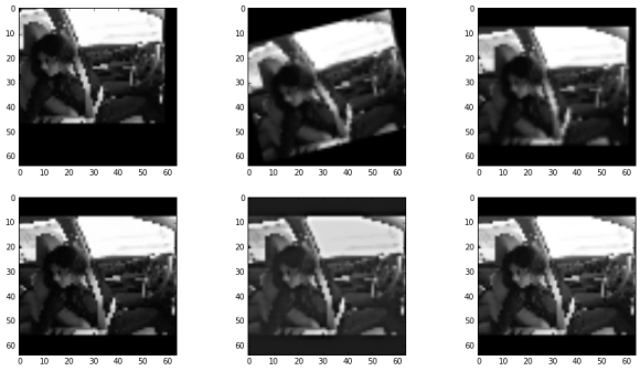
First, I’ll start with my assumptions. I started with a 128×128 crop of the original images for fast training on my GTX 960 desktop. I also throw away the RGB dimensions and relied on the grayscale images since I thought color doesn’t really factor much into the problem. I used batch norm, dropout and leaky rectifier units for my convolutions. I have early stopping based on my validation set. I figured I can get back to these later, especially on the matter of image sizes.
I used nolearn and lasagne for my solutions. I set aside a 40 images per class as my validation set. The training set now numbers 22,000. Data augmentation scales up this number to some hundreds of thousands since I use the following augmentation operations: Translation, rotation, zooming, JPEG compression, sharpening and gamma correction. I did not do flips because the orientation of all the images are the same.
I used a modified VGGNet architecture for most of my models. I emphasized on coverage and capacity, as a heuristic for my convolutional stacks. I used L2 normalization with a value of 5e-4. Here’s how it looks like:
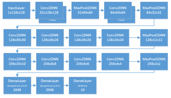
With this, I achieved a 1.05 cross entropy validation loss and 1.18 public leaderboard score. Not bad, but could be better. I also noticed that I am achieving a clean 100% accuracy for my validation set, but a rather high loss. So I figured that this would be a battle of regularization.
I resubmitted the same architecture but with an L2 normalization parameter of value 5e-3. This results in a more regularized model, but with a slightly worse fit for the training set. This results in a significantly better validation loss of 0.285 and public leaderboard score of 0.916.
I missed something!
Reviewing my architecture, I forgot to add in batch norm for my dense layers. During my readings from deep learning literature, I also come across the advantages of orthogonal weight initialization. I add both in, while also adding an extra convolutional stack before the dense layer. It looks like this:
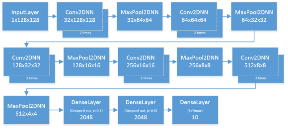
This results in a very satisfying validation loss of 0.236 and public leaderboard score of 0.352. This is my best single model. Very satisfied, I set this as one of my final submissions.
Maxout and ensembles
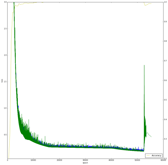
I used maxout for my dense layers as my final model architecture. All parameters being equal, this model has a maxout layer with k=8 for my two dense layers. I had a better validation loss of 0.18, however, this ended up at a disappointing 0.3811 public leaderboard score. I reviewed the training history and noticed that my learning rate schedule of three steps (decrease learning rate by a magnitude of 10 every 8,000 minibatches) was too aggressive and hindered learning. Notice below the point between 10k and 20k where the training loss plateaued. I revised the schedule of having only two steps, 0.001 from 0 to 8k, and 0.0001 onwards. I achieved a lower validation loss, but my public leaderboard standing remained the same.
My last single model involved an image size of 261×261 with my maxout architecture. It achieved a validation score of 0.174 but its leaderboard score is 0.571. I figured my learning rate was set wrong since training with a larger image would need a different schedule as a smaller one. I need more time!
With the deadline coming near, I decided to simply use an ensemble model, using my best model and my maxout models, not including the 261×261 predictions. It achieved a better leaderboard score of 0.302, and it propelled me to top 200!
Learnings
I am very satisfied with this placing and it enabled me to learn so much, especially for my other projects. Some key learnings:
- Tune the learning rate properly. This is a very basic technique, but one that is very critical for training large networks.
- Smaller image sizes train fast, but always leave time for training larger ones. Man, I wish I did this earlier.
- It’s very hard to learn from scratch. It was only after the competition deadline where I thought of simply using transfer learning to get a pretrained model and start from there.
- When using batch norm, don’t forget to include the dense layers!
- Ensemble predictions do well, so always leave time for storing all the output probabilities to use later. Maybe one can also tune the weights of their predictions as in a weighted bagging scheme.
With that, I thank State Farm for the great competition. Congratulations to the winners! I see the top two finalists are soloists. Impressive!
As for me, when the private leaderboards was released I dropped to #235, using my ensemble model. It’s my highest final leaderboard standing in Kaggle though (top 17%)! I’ll upload my solutions in a while.
Thanks for reading!
