
Hey all, it’s time for another machine learning blog. This time, I’m tackling recommendation systems. I’ve found this neat dataset, Steam Video games over at Kaggle. You should definitely check it out. We’ll be going from analyzing how people play these games, to how we can infer ratings from usage patterns. I’ll be implementing my own recommendation algorithm, and then using the current state-of-the-art. Lastly, we’ll be finishing up with describing the bleeding edgeo
For non-gamers out there, Steam is a video game platform that’s both a marketplace and a community. Big and small vendors can sell their content here and players choose from thousands of available titles.
Loading up the dataset
import numpy as np
import pandas as pd
%pylab inline

data = pd.read_csv("data/steam-200k.csv", header=None, index_col=False,
                   names=["UserID", "GameName", "Behavior", "Value"])
data[:5]
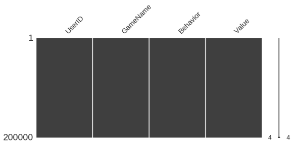
import missingno as msno
msno.matrix(data, figsize=(10,4))
# no missing values!
Going Descriptive
There are many more users than games. This is a common trait for many datasets. But note that there may be other cases where the items outnumber the users. WordPress and Youtube come to mind!
print("Data shape: ", data.shape)
print("Unique users in dataset: ", data.UserID.nunique())
print("Unique games in dataset: ", data.GameName.nunique())
So people purchase on average 10 games… But play 48 hours on average for each! What a lucrative market!
Some outliers are plain funny:
- A person bought 1000+ games. Really.
- What’s up with the person who did 11k hours of gaming? That’s ~450 days!
# average number of games per user
games_transacted = data.groupby("UserID")["GameName"].nunique()
games_purchased = data[data.Behavior == "purchase"].groupby("UserID")["Value"].sum()
games_played = data[data.Behavior == "play"].groupby(["UserID","GameName"])["Value"].sum()

print("Games Transacted Stats:")
print(games_transacted.describe())

print("Games Purchased Stats:")
print(games_purchased.describe())

print("Games Played Stats:")
print(games_played.describe())
So in Graphical Terms, this is how it looks like
Let’s remove outliers, that is, those with mean +sd*4.
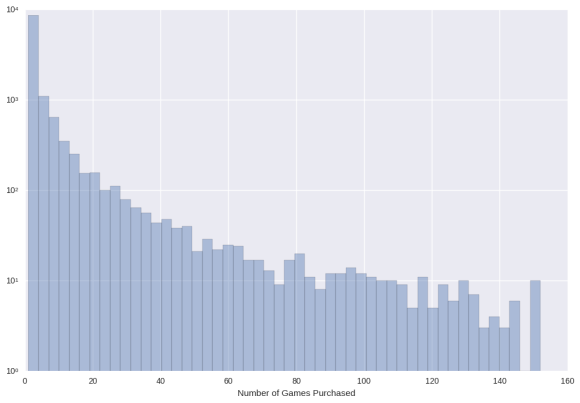
Games Bought
It looks another showing of the power law, but with a gentler slope. People just seem to buy a lot of games.
import seaborn as sns
f, ax = plt.subplots(figsize=(12, 8))
mean_v = np.mean(games_purchased)
std_v = np.std(games_purchased)
inliers = games_purchased[games_purchased < mean_v + 4* std_v]

sns.distplot(inliers, ax=ax, axlabel="Number of Games Purchased", kde=False)
ax.set(yscale="log")
plt.show()
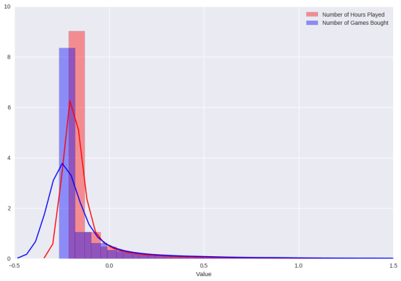
Does the distribution of bought games look like the hours spent?
In other words, are the bought games worth it in terms of hours?
To answer this, we must standardize the two variables so we can compare them on the same scale.
Studying the graph below, it does seem that it is worth it. People as a whole seem to spend time with their bought games. More precisely, people spend more time with their games more than they purchase them.
def standardize(series):
    return (series - np.mean(series)) / np.std(series)

f, ax = plt.subplots(figsize=(12, 8))
games_played_standardized = standardize(games_played)
mean_v = np.mean(games_played_standardized)
std_v = np.std(games_played_standardized)
games_played_inliers = games_played_standardized[games_played_standardized < mean_v + 4* std_v]

sns.distplot(games_played_inliers, ax=ax, label="Number of Hours Played", color="red")

games_purchased_standardized = standardize(games_purchased)
mean_v = np.mean(games_purchased_standardized)
std_v = np.std(games_purchased_standardized)
games_purchased_inliers = games_purchased_standardized[games_purchased_standardized < mean_v + 4* std_v]

sns.distplot(games_purchased_inliers, ax=ax, label="Number of Games Bought", color="blue")

plt.legend()
ax.set_xlim(-0.5, 1.5)
plt.show()
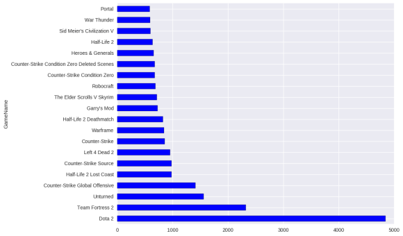
What are the most popular games?
And why Valve can’t count to 3.
# in terms of purchases
game_purchases = data[data.Behavior == "purchase"].groupby("GameName")["Value"].sum()
plt.figure(figsize=(10,8))
game_purchases.sort_values(ascending=False)[:20].plot(kind="barh")
plt.show()
# in terms of play time
game_plays = data[data.Behavior == "play"].groupby("GameName")["Value"].sum()
plt.figure(figsize=(10,8))
game_plays.sort_values(ascending=False)[:20].plot(kind="barh")
plt.show()
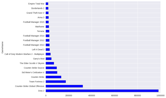
Dota 2 is life! It’s free to play but a lot of people purchased/installed it.
# for the top 10 most purchased games, what is the distribution of their play times?
top_10_most_purchased = game_purchases.sort_values(ascending=False)[:10].index.tolist()
top_10_most_purchased_playhours = data[(data.GameName.isin(top_10_most_purchased)) & (data.Behavior == "play")]
ax = sns.boxplot(x="GameName", y="Value", data=top_10_most_purchased_playhours)
plt.xticks(rotation=90)
ax.set(yscale='log')
plt.show()
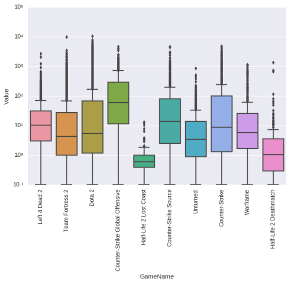
CSGO takes the win on this one. Although there are a few very dedicated individuals in Dota 2 and Team Fortress 2.
And indeed Valve can’t count to three. Gaben plz.
Let’s make a rating system
Say, a purchase of a game is a rating of 1. The number of hours playing a game determines the rating for the game, as determined by both global percentiles and a weighting scheme I’ll describe below.
# let's take care of the 1 ratings first
purchase_ratings = data[data.Behavior == "purchase"].groupby(["UserID", "GameName"])["Value"].count()
purchase_ratings.describe()
What? Why are there bought games with count two? Turns out with the user below, he can indeed buy things twice. And there’s sizable data about this. For now, let’s park this phenomenon and review it later.
purchase_ratings[purchase_ratings > 1][:5]
purchase_ratings[purchase_ratings > 1].shape
# making every value a 1
purchase_ratings[purchase_ratings > 1] = 1
Number of hours played
Now, for the number of hours played, we’ll base each rating for each game as a function of three variables:
= user i played hours
= nth percentile of population played hours with respect to game j
= user’s total games played
We want users who has played the game in say the, 75th percentile of population played hours with respect to that game to have high scores.
On the other hand, if a game j is the only game the player plays, then his played hours should be counted as more valuable as opposed to users that play a lot of other games. So we weight in the following manner:

where alpha is the global mean parameter.
We then compute the percentiles $p_{j}^{(n)}$ over this new weighted space and call it 
With this, when the number of the games of a user is below the global mean, then her played hours is weighted up. Conversely, if the number of games of a user is above the global mean then her played hours is weighted down.
Then, to transform to ratings, one considers percentiles.

games_played_per_user = data[data.Behavior=="play"].groupby(["UserID"])["GameName"].nunique()

average_games_played = games_played_per_user.mean()
weighted_games_played = games_played * (average_games_played / games_played_per_user)

def to_explicit_ratings(series):
    games = series.index.levels[1].tolist()
    hours_ratings = series.copy()
    for game_played in games:
        sliced_data = hours_ratings.xs(game_played, level=1)
        descr = sliced_data.describe()
        a = sliced_data[sliced_data >= descr["75%"]].index.tolist()
        hours_ratings.loc[(a, game_played)] = 5
        b = sliced_data[(sliced_data >= descr["50%"]) & (sliced_data < descr["75%"])].index.tolist()
        hours_ratings.loc[(b, game_played)] = 4
        c = sliced_data[(sliced_data >= descr["25%"]) & (sliced_data < descr["50%"])].index.tolist()
        hours_ratings.loc[(c, game_played)] = 3
        d = sliced_data[sliced_data < descr["25%"]].index.tolist()
        hours_ratings.loc[(d, game_played)] = 2

    return hours_ratings

hours_ratings = to_explicit_ratings(weighted_games_played)
mean_weighted_ratings = purchase_ratings.combine(hours_ratings, max)
print mean_weighted_ratings.shape
print mean_weighted_ratings.describe()
sns.distplot(mean_weighted_ratings, kde=False)
plt.show()
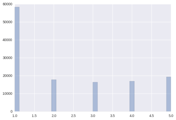
So now we have our ratings. We have to ask though, what’s the effect of weighting?
Note that the mean is 6.209427 and the standard dev is 17.754906.
Before and after
What happens with these three users?
- User 62990992 is the most active with 498 games played.
- User 16081636 has played 25 games, one SD above the average
- User 309167186 has played a single game, but has spent only 1.1 on it.
def display_before_and_after(user_id, before, after):
    print "====Before===="
    games_played = min(len(non_weighted_ratings.ix[user_id]), 10)
    idx = before.xs(user_id, level=0).sample(games_played).index.tolist()
    print before.xs(user_id, level=0)[idx]
    print "====After===="
    print after.xs(user_id, level=0)[idx]
non_weighted_ratings = to_explicit_ratings(games_played)
non_weighted_ratings = purchase_ratings.combine(non_weighted_ratings, max)
display_before_and_after(62990992, non_weighted_ratings, mean_weighted_ratings)
display_before_and_after(16081636, non_weighted_ratings, mean_weighted_ratings)
display_before_and_after(309167186, non_weighted_ratings, mean_weighted_ratings)
# cleanup
purchase_ratings = None
hours_ratings = None
data = None
Let’s finally model
We’ll first establish how to evaluate our recommendations — train and test. Then we’ll implement a user-based k-nearest neighbors algorithm.
ratings = mean_weighted_ratings.reset_index()
ratings.rename(columns={0:"Rating"}, inplace=True)
print(ratings.shape)
from scipy.spatial.distance import cosine

def get_similarity(r, user_1, user_2):
    return list(set(r[r.UserID == user_1]["GameName"]).intersection(r[r.UserID == user_2]["GameName"]))

def compute_distance(r, user_1, user_2, items_both_rated = 3):
    similar_items = get_similarity(r, user_1, user_2)
    if not similar_items:
        return np.inf
    if len(similar_items) < 3:
        return np.inf
    vector_1 = r[(r.UserID == user_1) & r.GameName.isin(similar_items)]\
                    .sort_values("GameName")["Rating"].values
    vector_2 = r[(r.UserID == user_2) & r.GameName.isin(similar_items)]\
                    .sort_values("GameName")["Rating"].values

    return cosine(vector_1, vector_2)

def get_closest_users(r, user_1, threshold = 0.001, items_both_rated = 3, sample_frac = 1.0):
    others = pd.Series([v for v in set(r.UserID) if v != user_1]).sample(frac=sample_frac)
    neighborhood = []
    for other in others:
        distance = compute_distance(r, user_1, other, items_both_rated=items_both_rated)
        if distance <= threshold:
            neighborhood.append((other,1-distance))
    return neighborhood
neighborhood = get_closest_users(ratings, 5250)
print len(neighborhood)
print neighborhood[:10]
Let’s see if 5250 and 17531316 are similar. Seems like 5250 collected almost Valve games, but didn’t play those games much. Seems like he likes shooter games, with Deus Ex, Alien Swarm, Portal and Team Fortress in the list.
186517004 on the other hand, looks like a first-person shooter expert with Call of Duty and CSGO leading his list.
ratings[ratings.UserID == 5250]
ratings[ratings.UserID == 186517004]
User-Based K-Nearest Neighbors Recommender
 $
$from collections import defaultdict
def novel_items_from_user(r, user_1, user_2):
return list(set(r[r.UserID == user_2]["GameName"]).difference(r[r.UserID == user_1]["GameName"]))
def k_nearest_neighbors_user_recommender(r, user_1, n_ratings=None, items_both_rated=3,
threshold=0.005, nh_size=20, sample_frac=1.0):
neighborhood = get_closest_users(r, user_1, items_both_rated=items_both_rated, threshold=threshold,
sample_frac=sample_frac)
neighborhood.sort(key=lambda x: x[1], reverse=True)
if nh_size:
neighborhood = neighborhood[:nh_size]
novel_items = []
for (neighbor, similarity) in neighborhood:
n = novel_items_from_user(r, user_1, neighbor)
novel_items.extend(n)
running_dict = defaultdict(list)
for (neighbor, distance) in neighborhood:
item_id_rating = r[(r.UserID == neighbor) & (r.GameName.isin(novel_items))][["GameName", "Rating"]]
for (item_id, rating) in item_id_rating.to_records(index=False):
running_dict[item_id].append((similarity * rating) / similarity)
for item in running_dict:
running_dict[item] = sum(running_dict[item]) / len(running_dict[item])
recommendations = running_dict.items()
recommendations.sort(key= lambda x: x[1], reverse=True)
if n_ratings:
return recommendations[:n_ratings]
else:
return recommendations
%%time
user_id = 5250
novel_items = k_nearest_neighbors_user_recommender(ratings, user_id)
novel_items[:20]
The thing is, it takes a long time to compute recommendations for a single user. This is because user-based recommenders require a neighborhood to be computed. A quick optimization should be to sample N users to create a neighborhood.
%%time
user_id = 5250
novel_items = k_nearest_neighbors_user_recommender(ratings, user_id, sample_frac=0.5)
novel_items[:20]
The results are not bad with 5250 being recommended Left 4 Dead, Crysis, XCOM. Very intuitive results.
Calling Libraries
There are libraries out there that have plenty of contributors. Such is the power of open-source. The standard algorithms are already implemented. I’ll use here scikit-surprise , which is both a framework and repository of standard algorithms. We’ll be comparing SlopeOne and SVD here.
SlopeOne is an item-based recommendation algorithm that uses the differences of item ratings across the users. It’s an attractive algorithm because the evaluation part of the algorithm is very fast. Computation doesn’t depend on the number of users. However, it does have a lengthy precomputation phase.
SVD is the algorithm that won the Netflix prize. The ratings matrix is decomposed into Q and P matrices, plus some biases that account for each user’s and item’s expected rating. Computation involves gradient descent, so it is computationally intensive. The ratings are modeled by the following function:

ratings.to_csv("data/steam-200k-weighted-ratings.csv", index=False, sep='\t')
from surprise import SVD, SlopeOne
from surprise import Dataset, Reader
from surprise import evaluate, print_perf

reader = Reader(line_format='user item rating', sep='\t', skip_lines=1)
data = Dataset.load_from_file("data/steam-200k-weighted-ratings.csv", reader)
data.split(n_folds=10)

algo = SlopeOne()

# Evaluate performances of our algorithm on the dataset.
perf = evaluate(algo, data, measures=['RMSE', 'MAE'])

print_perf(perf)
algo = SVD(lr_all=0.001)

# Evaluate performances of our algorithm on the dataset.
perf = evaluate(algo, data, measures=['RMSE', 'MAE'])

print_perf(perf)
So we have Matrix Factorization as the winner by ~0.03 points. It may not seem much but this improvement marks the difference between \$ and \$$$!
Final Thoughts
Recommendation is arguably one of the most commercial applications of machine learning. With the successes of Netflix, Youtube and Outbrain, algorithmists have been thinking of ways to predict the elusive idea of a person’s interest. As seen in Netflix’s results, recommendations have come close to reverse engineering Hollywood. And it will only get better at discovering our interests. Right now, we’ve only handled user interactions across the site. This is called collaborative filtering. Its close relative is analyzing item characteristics. This is called content-based filtering. Both are good in some respects, but they have weaknesses.
To go deeper, we need more. More computation and more context. The bleeding edge of recommendation systems, I believe, hinges on these two requirements. Factorizing machines have k-dimensional latent vectors associated with each variable (i.e. users and items). This algorithm can potentially uncover more complex interactions than collaborative/content-filtering and SVD. For more on this algorithm, head on over to https://getstream.io/blog/factorization-machines-recommendation-systems/
Lastly, more context. Deep learning has allowed us to see inside the video itself. Rather than use annotations (manual or automated) for content-based filtering, deep learning has the potential to go beyond annotations and enable the video to be “seen” by a “neural network’s eyes”. We’re now crossing to computer vision territory. As proof of its potential, Youtube has already implemented deep learning across search and recommendation. For more, read up on this paper https://research.google.com/pubs/pub45413.html.
That’s about it. Thanks for reading.

2 replies on “Steam Games Recommender”
[…] out my other post for my previous shot at […]
LikeLike
[…] Memory-based recommendation – I implement from scratch […]
LikeLike