Collaborative Denoising Autoencoders on Steam Games

Recommendation systems are ubiquitous in our digital lives. To improve the quality of the recommended items, researchers have proposed hundreds of algorithms to the existing literature. Many have found their way to large production systems while new breeds of algorithms are being developed and tested all the time.

In this post, I am introducing the collaborative denoising autoencoder by Yao et al and trying it on the steam-games dataset. CDAE is a variant of an autoencoder that is well-suited for the recommender domain. Let’s tackle some preliminaries first:

• Autoencoders are neural networks that try to learn a compressed mapping from the input. It does this by first, forcing the input to an information bottleneck (encoder) and then trying to recreate the original input from the compressed representation (decoder).
• Bottlenecks come in many forms, such as far fewer nodes in the hidden layer, adding noise to the input, having a regularization term in the loss function, or a combination of many techniques.
• Typically, autoencoders are used to pre-train large networks, since it does not require additional labels from the data. It uses the data itself for training — what is called self-supervised learning.

Autoencoders are very interesting for recommendation since it has the capacity to learn an efficient lower-dimensional representation from the input. This is very related to matrix factorization, which learns a latent representation of users and items from the ratings matrix. Matrix factorization is the workhorse of many recommender systems and efforts to improve, generalize, reframe, and even reinvent this wheel are very attractive for researchers and engineers. In recommendation, the input is very sparse (the long tail problem) and CDAE may be one way to tackle sparsity.

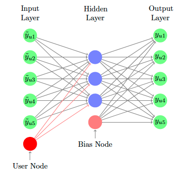
CDAE has the following architecture. The input layer has a user node (in red) which enables user-personalized information to flow through the network. The hidden layer has significantly fewer nodes than the inputs and the outputs. This is similar to the idea of the number of latent dimensions in matrix factorization and in principal components analysis. Training the network involves corrupting the inputs by some amount and forward passing it through the network. The output layer must approximate the inputs even though there is an information bottleneck AND corrupted data. This makes the network create an effective lower-dimensional mapping of the ratings. For inference, the input is not corrupted and does a forward pass through the network. The n highest outputs form the top-n recommended items.

Sidebar: Other blogs

A quick aside. I also refer you to my other blog posts on the steam games dataset. I like this dataset since I can relate to many of the games — just like you!

• Memory-based recommendation – I implement from scratch
• Explainability in recommendation – I used the implicit library

Implementation

For my implementation, I am attributing a lot to the work of James Le’s code and his article. I also recommend RecBole for the reader to study.

I am using Pytorch Lightning to structure my code. Ray Tune is used for hyperparameter optimization. CometML is used to log my results. You can go to my Kaggle Notebook here, and the CometML Experiment here.

The Data and its DataLoader

The steam games dataset contains purchase and play user behaviors for thousands of games. In this exercise, we convert all purchases / plays to 1. All items and users with ratings less than 4 are removed iteratively. It resulted in the following ratings matrix. It’s small but good enough for a demo.

Before thresholding interactions
Number of users: 12393
Number of items: 5155
Number of rows: (128804, 3)
Density: 0.0020161564563957487
After
Starting interactions info
Number of rows: 12393
Number of cols: 5155
Density: 0.202%
Ending interactions info
Number of rows: 4377
Number of columns: 2959
Density: 0.881%
Number of users: 4377
Number of items: 2959
Number of rows: (114089, 3)
Density: 0.008808911803018373

For the data splits, I did the following: Users with more than 5 ratings had 20% of their ratings become part of the validation set. I repeat this process for the test set.

After data preparation, I spin up data loaders for PyTorch. We have three versions — train, test, and inference. The train loader contains the sparse matrix for training. The test loader contains the training matrix and the target matrix. The inference loader contains the user ids for inference. If we don’t do this, then our user id indexes are computed from the provided sparse matrix of behaviors instead of the original input space.

	class RecoSparseTrainDataset(Dataset):
	def __init__(self, sparse_mat):
	self.sparse_mat = sparse_mat
	def __len__(self):
	return self.sparse_mat.shape[0]
	def __getitem__(self, idx):
	batch_matrix = self.sparse_mat[idx].toarray().squeeze()
	return batch_matrix, idx
	class RecoSparseTestSet(Dataset):
	"""
	The test dataset contains the training and test matrices.
	The latter should be predicted from the training
	"""
	def __init__(self, train_mat, test_mat):
	self.train_mat = train_mat
	self.test_mat = test_mat
	assert train_mat.shape == test_mat.shape
	def __len__(self):
	return self.train_mat.shape[0]
	def __getitem__(self, idx):
	train_matrix = self.train_mat[idx].toarray().squeeze()
	test_matrix = self.test_mat[idx].toarray().squeeze()
	return train_matrix, test_matrix, idx
	class RecoSparseInferenceDataset(Dataset):
	def __init__(self, sparse_mat, user_ids):
	"""
	sparse_mat : interaction matrix
	user_ids : ids of the users (positional)
	"""
	self.sparse_mat = sparse_mat
	self.user_ids = user_ids
	assert sparse_mat.shape[0] == len(user_ids)
	def __len__(self):
	return self.sparse_mat.shape[0]
	def __getitem__(self, idx):
	batch_matrix = self.sparse_mat[idx].toarray().squeeze()
	batch_ids = self.user_ids[idx]
	return batch_matrix, batch_ids
	###
	batch_size = 512
	num_workers = multiprocessing.cpu_count()
	train_loader = torch.utils.data.DataLoader(RecoSparseTrainDataset(train), batch_size=batch_size, shuffle=True, num_workers=num_workers)
	val_loader = torch.utils.data.DataLoader(RecoSparseTestSet(train, val), batch_size=batch_size, shuffle=False, num_workers=num_workers)
	test_loader = torch.utils.data.DataLoader(RecoSparseTestSet(train, test), batch_size=batch_size, shuffle=False, num_workers=num_workers)

view raw cdae_dataloaders.py hosted with ❤ by GitHub

The Model

PyTorch Lightning requires some simple object-oriented programming rules to structure the training loop. The upside is enormous: A whole framework to lean on with various callbacks, loggers, scheduling strategies, multi-GPU support, and others. I have the following gist for you to check out, but please check the entirety of the class here.

	class CDAE(pl.LightningModule):
	def __init__(self, model_conf : Dict, novelty_per_item, num_users, num_items, remove_observed = False, ):
	super().__init__()
	self.hidden_dim = model_conf["hidden_dim"]
	# … other self. initializations
	self.user_embedding = nn.Embedding(self.num_users, self.hidden_dim)
	self.encoder = nn.Linear(self.num_items, self.hidden_dim)
	self.decoder = nn.Linear(self.hidden_dim, self.num_items)
	self.criterion = nn.BCELoss(reduction='sum')
	# for flattened dictionary logging, add to conf
	model_conf["num_users"] = num_users
	model_conf["num_items"] = num_items
	self.save_hyperparameters(model_conf, ignore=["novelty_per_item", "remove_observed"])
	def forward(self, x):
	rating_matrix, user_idx = x
	# … some normalize options here
	# …
	# (1) corrupt the rating matrix when in training
	corrupted_rating_matrix = F.dropout(rating_matrix, self.corruption_ratio, training=self.training)
	# (2) build the collaborative denoising autoencoder
	# first term – ratings, second term – user embedding
	embedded_users = self.user_embedding(user_idx)
	encoded_ratings = self.encoder(corrupted_rating_matrix)
	enc = torch.add(embedded_users, encoded_ratings)
	enc = self.__apply_activation(self.act, enc)
	dec = self.decoder(enc)
	return self.__apply_activation(self.out_act, dec)
	def training_step(self, batch, batch_idx):
	# negative sampling options here
	# …
	pred_matrix, batch_matrix = self.__get_pred_matrix(batch, batch_idx)
	loss = self.criterion(pred_matrix, batch_matrix)
	# logs metrics for each training_step,
	# and the average across the epoch, to the progress bar and logger
	self.log("train_loss", loss, on_epoch=True, prog_bar=True, logger=True)
	return loss
	def validation_step(self, batch, batch_idx):
	score_prefix = "val"
	return self.__shared_evaluation(batch, batch_idx, score_prefix)
	def __get_pred_matrix(self, batch, batch_idx):
	batch_matrix, user_ids = batch
	pred_matrix = self(batch)
	return pred_matrix, batch_matrix
	def __shared_evaluation(self, batch, batch_idx, prefix):
	with torch.no_grad():
	train_matrix, test_matrix, user_ids = batch
	pred_matrix = self((train_matrix, user_ids))
	# compute loss on targets
	loss = self.criterion(pred_matrix, test_matrix)
	# (1) convert test matrix to dictionary
	targets = np_mat_to_dict(test_matrix.cpu().numpy())
	# (2) Get the top-k predictions
	pred_matrix = pred_matrix.cpu().numpy()
	top_k_recos = self.predict_topk(pred_matrix, self.max_k)
	# (3) Precision, Recall, NDCG @ k
	scores = self.__prec_recall_ndcg(top_k_recos, targets)
	# … and other metrics
	# …
	self.log_dict(score_dict, on_epoch=True, prog_bar=True, logger=True)
	return score_dict

view raw cdae_model_short.py hosted with ❤ by GitHub

To train, we use the CometML & Ray Tune duo. The former collects the metrics via CometLoggerCallback. The latter does the hyperparameter tuning with a few added lines only. In this exercise, the parameters are exhaustively used through grid search. If you need something smarter, then there are other search algorithms to try, as well as a time budget to constrain costs if needed.

	# pip install ray tune, and comet ml
	from ray.tune.integration.comet import CometLoggerCallback
	from functools import partial
	from ray.tune.integration.pytorch_lightning import TuneReportCallback
	def train_function(model_conf, novelty_per_item, epochs, patience,
	train_loader, val_loader, checkpoint_dir=None):
	model = CDAE(model_conf, novelty_per_item, num_users, num_items)
	# fill up your metrics here
	metrics = ["val_loss_epoch",
	"val_Prec@20"]
	# this is needed so ray tune and PyTorch can communicate
	raytune_callback = TuneReportCallback(metrics, on="validation_end")
	callbacks = [pl.callbacks.EarlyStopping("val_loss_epoch", mode='min', patience=patience),
	raytune_callback]
	trainer = pl.Trainer(accelerator="auto", callbacks=callbacks, max_epochs=epochs,
	enable_progress_bar = False, log_every_n_steps=1)
	trainer.fit(model=model, train_dataloaders=train_loader, val_dataloaders = val_loader)
	# this is the search space
	search_space_conf = {
	"hidden_dim": tune.grid_search([50, 100, 200]),
	"corruption_ratio": tune.grid_search([0.3, 0.5, 0.8]),
	"activation": tune.grid_search(['sigmoid', 'tanh']),
	"negative_sample_prob": tune.grid_search([0, 0.5, 1]),
	"learning_rate": tune.grid_search([0.1, 0.05, 0.01]),
	"wd": tune.grid_search([0, 0.01, 0.001]),
	}
	# this is the callback
	comet_logger = CometLoggerCallback(
	api_key=API_KEY,
	project_name=PROJECT_NAME,
	workspace=WORKSPACE,
	tags=["cdae_tuning"]
	)
	train_function_instance = partial(train_function, model_conf, novelty_per_item,
	epochs, patience, train_loader, val_loader, )
	analysis = tune.run(
	train_function_instance,
	name='cdae',
	metric="val_Prec@20",
	mode='max',
	config=search_space_conf,
	callbacks=[comet_logger],
	# time_budget_s=200
	)

view raw cdae_tune.py hosted with ❤ by GitHub

Model Results

CometML produces some of the most beautiful panels I’ve seen in machine learning. You can graph your parameters against metrics, collaborate with others through notes, and have a model registry for your team as well. Definitely worth checking out. Isn’t the following dashboard amazing? This is from the hyperparameter tuning that we’ve done above.

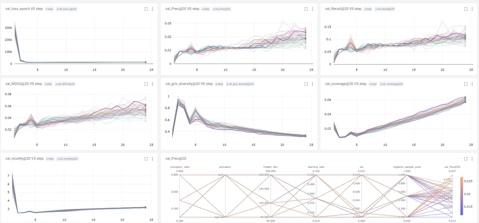
The parallel coordinates chart on the bottom right informs how the hyperparameter search ended up with the best model. I ended up with the hyperparameters below. In this exercise, the number of hidden nodes and the corruption ratio are the most crucial influencing factors for the final metrics.

{'hidden_dim': 200, 'corruption_ratio': 0.3, 'activation': 'sigmoid', 'negative_sample_prob': 0, 'learning_rate': 0.01, 'wd': 0.001}

For the metrics, some of these should be familiar. These metrics are parametrized @ k, which are the first k recommended items. Precision and recall are similar to precision and recall in the classification setting. NDCG is a measure of ranking quality. The following are some metrics “beyond” accuracy:

• Gini diversity – a measure of the difference of recommended items across users. The lower, the more unique the recommendations.
• Coverage – how many items are being recommended over the total items in the train set
• Novelty – a metric that captures how popular the first k recommendations are. The lower, the more “unsurprising” the recommendations.

Metrics for k=20	Value
Precision	0.026
Recall	0.194
NDCG	0.072
Gini Diversity	0.267
Coverage	0.202
Novelty	3.921

Sample Recommendations

Now for the fun part — the actual games! Each of my examples below is captioned with some sort of reasoning on why it could be a good or bad recommendation. With this type of evaluation, it can get very subjective, but you can get a good sense of what the model is doing.

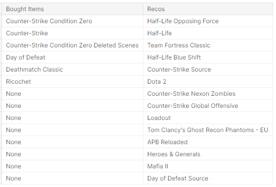
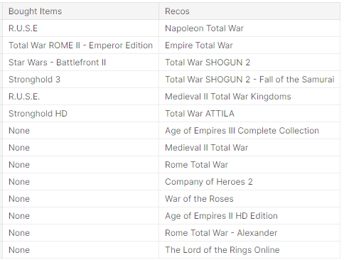
What do you think? Does it make sense?

Where do we go from here?

At this point, you may have a good sense of how autoencoders can work in the recommendation setting. This is arguably one of the simplest algorithms in this space, but you should also try out Variational Autoencoders and Sequence Autoencoders.

You can also upgrade your work from a notebook to an MLOps pipeline. MLOps is all about creating sustainability in machine learning. Consider that you have a dozen projects, models, training loops, serving pipelines… Clearly, a framework is needed to organize things. Kedro is one way to manage all of that.

Lastly, I have also written a project where I implement a recommendation pipeline from data engineering, to training, testing, and deployment. It’s a lengthy process, but well worth it to make your ML sustainable.

Thanks for reading!