
In this post, I’m using the implicit library by Ben Frederickson , a well-designed Python library that computes recommendations from implicit feedback. This time, I’ll be focusing on explaining recommendations, which is a big part of a user’s experience. Often, recommendations are printed as “You Might Like X because you watched Y.” This connection grounds the user from a prior experience and encourages her to consume the recommended content.
The foundations of this post is the much cited work of Yifan Hu, Collaborative Filtering for Implicit Feedback Datasets. On Section 5, it explains how the latent factors could be used to explain recommendations. More on that later.
I’ll be using the Steam Video Games dataset from Kaggle. It’s a small dataset and it’s no secret that video games is another hobby of mine.
Check out my other post for my previous shot at this.
import numpy as np
import pandas as pd
%pylab inline

data = pd.read_csv("data/steam-200k.csv", header=None, index_col=False,
                   names=["UserID", "GameName", "Behavior", "Value"])
data[:5]
print "Data shape: ", data.shape
print "Unique users in dataset: ", data.UserID.nunique()
print "Unique games in dataset: ", data.GameName.nunique()
# average number of hours spent per game
hours_played = data[data.Behavior == "play"].groupby(["UserID","GameName"])["Value"].sum()
print("Hours Played Stats:")
print(hours_played.describe())
import seaborn as sns

sns.distplot(hours_played[hours_played < 1000])
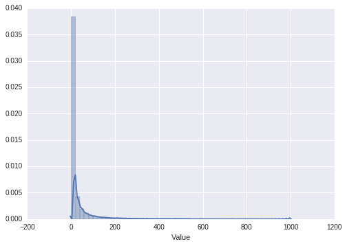
Some Preprocessing
1) This dataset is small, 200k rows, with 12k users and 5k games.
2) A behavior of “play” and its corresponding “Value” indicates the number of hours playing the game.
3) As you can see, the hours played is highly skewed to the right with some hardcore players consuming too much hours.
4) Since we’re using implicit feedback, outliers may skew the results to very popular games. I’ll introduce tukey’s method to clip the outliers. Other methods include BM-25, which I’ll get to in a while.
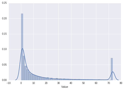
hours_played = hours_played.reset_index()
# tukey with k=3
k = 3

q75 = hours_played["Value"].quantile(0.75)
q25 = hours_played["Value"].quantile(0.25)
iqr = q75 - q25

hours_played["Value"] = hours_played["Value"].clip(0, q75 + iqr * 3)
sns.distplot(hours_played["Value"])
Some data transformation
The library requires the sparse format. This data structure is very memory-effective and offers some nice computation speedups as well.
You’ll also notice that the computation is very fast. As said in the paper, weighted matrix factorization runs in 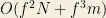
from scipy.sparse import coo_matrix

hours_played["UserID"] = hours_played.UserID.astype('category')
hours_played["GameName"] = hours_played.GameName.astype('category')

plays= coo_matrix((hours_played.Value.astype(np.float),
    (hours_played["GameName"].cat.codes.copy(),
    hours_played["UserID"].cat.codes.copy())) )
!export OPENBLAS_NUM_THREADS=1
import logging
logging.basicConfig(level=logging.DEBUG)
log = logging.getLogger("implicit")
log.setLevel(logging.DEBUG)
import implicit

model = implicit.als.AlternatingLeastSquares(factors=100, iterations=20, regularization=0.1,
                                             calculate_training_loss=True,
                                             num_threads=4)
model.fit(plays)
User recommendation
In WMF, recommendation involves multiplication of the latent factors. It turns out that with some clever manipulation of the user and item factors, one can explain the recommendations with the following linear expression.

The first factor in the summation is the weighted similarity of item i and j according to a user u’s viewpoint. The second factor is the confidence associated with user u’s past action. Another way of looking at it is that it is similar to neighborhood methods where similarities are immediately available. It’s just that now, we’re doing similarities of the latent factors and with the perspective of an input user. in As in the paper:
This shares much resemblance with item-oriented neighborhood models, which enables the desired ability to explain computed predictions... In addition,similarities between items become dependent on the specific user in question, reflecting the fact that different users do not completely agree on which items are similar.
Conveniently, the library already does this for us. There is an associated score for each recommendation, and each explanation also has a similarity score, the s in the above equation.
Let’s go for it!
user_to_id_mapping = dict([(user, idx) for (idx, user) in enumerate(hours_played.UserID.cat.categories)] )
id_to_user_mapping = dict(enumerate(hours_played.UserID.cat.categories))
item_to_id_mapping = dict([(item, idx) for (idx, item) in enumerate(hours_played.GameName.cat.categories)] )
id_to_item_mapping = dict(enumerate(hours_played.GameName.cat.categories))
def recommend_user(user_id, model, user_items, N=10, name=False):
    if name:
        return [(item_to_name_mapping[id_to_item_mapping[item]], score) for (item, score) in
            model.recommend(user_to_id_mapping[user_id], user_items, N=N)]
    else:
        return [(id_to_item_mapping[item], score) for (item, score) in
            model.recommend(user_to_id_mapping[user_id], user_items, N=N)]

def explain(user_id, model, user_items, N_recos=20, N_explanations=1, name=True):
    recos = recommend_user(user_id, model, user_items, N_recos, False)

    for item, score in recos:
        print("You might like:")
        print("'{}' ({}) because:".format(item, score))

        _, explanations, _ = model.explain(user_to_id_mapping[user_id],
                user_items, item_to_id_mapping[item], N=N_explanations)

        for related_item, weight in explanations:
            related_item_name = id_to_item_mapping[related_item]
            print("-- {} ({})".format(related_item_name, weight))
        print
User 1
1) Warhammer and Saint’s Row IV is explained clearly.
2) Alien vs. Predator is a little strange. Grand Theft Auto as well.
user_id = 87201181
user_items = plays.transpose().tocsr()
explain(user_id, model, user_items, N_recos= 5, N_explanations=2)
User 2
1) This user looks like a fan of action RPG.
2) Cities Skylines is strange however. A city-simulator connecting to an FPS is far-fetched.
user_id = 5250
user_items = plays.transpose().tocsr()
explain(user_id, model, user_items, N_recos= 5, N_explanations=2)
User 3
1) Here’s our fan of first-person shooters. Counter-strike is a good recommendation.
2) He also has a preference for strategy games, making RUSE a good recommendation.
user_id = 76767
user_items = plays.transpose().tocsr()
explain(user_id, model, user_items, N_recos= 5, N_explanations=2)
User 4
And here’s an RPG gamer.
user_id = 86540
user_items = plays.transpose().tocsr()
explain(user_id, model, user_items, N_recos= 5, N_explanations=2)
User 5
A Sportsman!
user_id = 17495098
user_items = plays.transpose().tocsr()
explain(user_id, model, user_items, N_recos= 5, N_explanations=2)
Conclusions
Some of the results were indeed helpful. I, in particular, liked the Football Manager recommendations. However I do have a few pointers:
1) Repeated recommendations of the same franchise should come less frequently. See those repeated Football Manager?
2) Steam has genre panes, for example, there is a pane for indie games, sports, RPG, FPS, strategy, etc. To fit these explanations per pane, one can add to the score another weight for genre similarity.
Thanks for reading.

One reply on “You Might Like… Why?”
[…] Explainability in recommendation – I used the implicit library […]
LikeLike